Political Analysis
Introduction
The modern American political landscape often seems void of bipartisanship. Nowhere is this stark divide between red and blue more evident than in the halls of the US Capitol, where the Senate and House of Representatives convene to carry out the duties of the legislative branch. While us average Americans rarely watch the daily proceedings of the Senate or House, Twitter has given us a unique window into the debates and discourse that shape our democracy. In fact, the 116th Congress, which served from January 3, 2019 to January 3, 2021 broke records by tweeting a total of 2.3 million tweets! As such, it is clear that Twitter is quickly becoming a digital public forum for American politicians. This surplus of tweets from the 116th Congress enables us to analyze the Twitter (following-follower) relationships between politicians on and across the two sides of the aisle. This project’s main inquiry is into whether there is a tangible difference in the way that Democrat members of Congress speak and interact on social media in comparison to Republican members of Congress. If there are such differences, this project will leverage them to train a suitable ML model on this data for node classification. That is to say, this project aims to determine a Senator’s political affiliation based off of a) their Twitter relationships to other Senators b) their speech patterns, and c) other mine-able features on Twitter. In order to truly utilize the complex implicit relationships hidden in the Twitter graph, we can use models such as Graph Convolutional Networks, which apply the concept of “convolutions” from CNNs to a graph network-oriented framework. These GCNs learn feature representations for each node in the Twitter graph and utilize those representations to fuel the aforementioned node classification task. However useful the GCN may be, there is no shortage of other graph ML techniques that could lend themselves to the prediction task at hand. Of particular interest are inductive graph ML techniques; inductive Graph Networks are a new assortment of Graph Networks that no longer need to be trained on a whole graph to get feature representations for all nodes in the dataset (transductive). Instead, inductive techniques like GraphSage peer into the structural composition of all the nodes in a graph by building neighborhood embeddings for each node. By using a medley of networks on this dataset, we gain deeper insight into what kind of graph we are working with. In other words, if more complex techniques like GraphSage outrank vanilla GCNs, it would point to an equally complex structural composition within the graph that only an inductive technique like GraphSage would be able to pinpoint. However, it is harder to train any network without features. In the case of our analysis, these features will be some text embedding of a politician's tweets. Solutions like word2vec or even a sentiment analysis metric that aggregate across the hundreds of thousands of tweets posted by the 116th Congress could prove quite useful as features for the training of the aforementioned models.
Datasets and Data Preprocessing
All the data we have collected are all scraped by ourselves from different websites. The main data sources are from two websites, one is twitter.com, and the other is from the United States Senate official website.
handles.csv
This dataset is a definitive mapping of each Senator’s Name, (Twitter) Handle, and Party
edges.csv
This dataset records Senatorial relationships on Twitter. For example, if Senator AK Lisa Murkowski followed UT Mitt Romney, this would be represented as “UT Mitt Romney” in the followed column and “AK Lisa Murkowski” in the following column. It has 3824 rows and 2 columns with two columns: followed and following. This data was gathered using the PhantomBuster Social Media Scraping API. The original dataset encompassed all Twitter accounts that each of these Senators followed, but this data was then filtered down to only Senator-Senator relationships.
tweets.csv
This dataset contains all Senatorial tweets during the 116th Congress (January 3, 2019 to January 3, 2021). It has 103428 rows and 3 columns : Senator Name, Tweet, Date Tweeted. This data was scraped using Twint, a python library for scraping from Twitter.
voting_data.csv
This dataset contains Senatorial voting patterns during the 116th Congress. This dataset contains the 79 bills that were issued by the Senate during their two years in session. It has 7900 rows and 3 columns: Senator Name, Decision, Bill. Each row represents how each Senator voted on a specific bill. There are four possible decisions for their vote: “Yea”, “Nay, “Not Voting”, “Absent”. This data was scraped from https://www.senate.gov using the python library beautifulsoup4.
voting_feature.csv
This dataset is created by ordinally encoding each of the aforementioned 4 possible votes and then pivoting the voting_data.csv. In this dataset, the bills being voted on represent the columns and each row represents how each Senator voted on each of the 79 bills. In total, it has 100 rows and 79 columns.
Exploratory Data Analysis
Figure 1: The visualization of edges.csv
Above is a visualization of the graph network scraped from Twitter. It is immediately apparent that the two political parties (Democrats being in blue, Republicans in red) are almost perfectly separated when visualized. This represents the very tangible divide that bifurcates the US Senate both in Twitter and in their voting patterns, as we will see later. We can also see that more far left members of the Senate, such as Senator Bernie Sanders, are in the bottom right of our graph. Meanwhile, Senator Josh Hawley, a Senator who openly supported the overturn of the 2020 presidential election is the red node in the upper left of the Figure. In this way, we can see that the graph network manages to convey not only the separation of the two parties, but also the alignments of some of these Senate members along the political spectrum. That is to say, the closer that a Senator is to the center of the graph, the more likely they are to be a political moderate. This assumption is further supported by an analysis of the closeness centrality of each of the nodes. Closeness centrality is a representation of how central a node is to a graph. More accurately, it is a sum of the shortest lengths between any node and the rest of the nodes in the graph. The node with the highest centrality would then represent the member of the Senate that is most connected with the opposite political party. In the case of the following network, the highest closeness centrality belongs to Democrat Senator Joe Manchin from West Virginia. This data makes sense in the context of the events following the inauguration of President Joe Biden, during which Manchin has repeatedly struck down proposals for a $15 minimum wage and ending the Senate filibuster (both of which are widely endorsed Democrat policies). Other Democrats who recently voted against the $15 minimum wage bill, such as Senator Margarent Hassan and Kyrsten Sinema, also have notably high centrality, which implies the relation between centrality and moderate political views. It is also worth noting that the average centrality of all Democrats (0.534007) is slightly higher than that of all Republicans (0.520566), implying that Democrats are more likely to interact with Republicans than vice-versa.
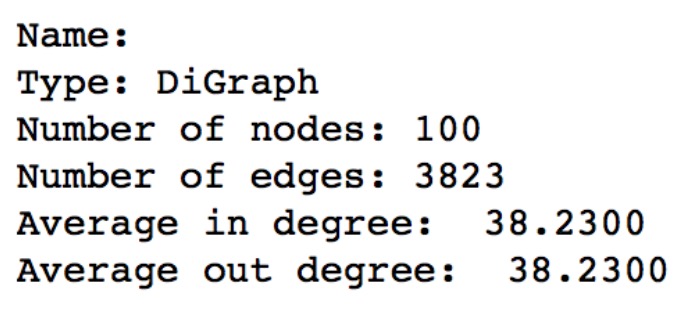
Figure 1: 2: Basic statistics for the graph network
The graph contains 3823 edges. The average in degree and out degree for the graph is 38.2300.
Methods
So far, we have implemented GCN and GraphSage as our cornerstone models for this project. The majority of the underlying codebase for these models is sourced from Yimei’s previous team: Group 2. Here is a brief detailing of how these two models work: We wrote these models in different .py files. The GCN model is in GCN_model.py and GraphSage is in graphsage.py. Our data is loaded from separate, organized files inside our project git. Our models and methods have demonstrated high performances for our classification task.
Data Loader
Our data is manually scraped from the internet, with the only automated portion being the scraping of Twitter follower-following relationships. The details of the datasets are already explained above. However, before we were capable of using this data, a great deal of cleaning was required to ensure that the Senator Names in all three tables matched (i.e. Solving discrepancies such as “Joe Manchin the III” vs. “Joe Manchin”) in order to ensure we could use names as a reliable primary key across all tables. After such cleaning, we created the three key tables listed above in a format suitable for quick use. Therefore, our data loader function is solely designed to load the datasets as is with minimal adulteration. This data loader, which accepts two file addresses as arguments, loads the feature dataset and edges dataset respectively. One is the address of the feature dataset, and another is the edges dataset. The current feature dataset (Voting Data) contains the matrix, which has 100 rows and 80 columns. The only transformations are 1) changing the label set from a categorical feature space to an ordinal feature space and 2) transforming the edges into an adjacency matrix. As such, the structure of the Data Loader is simple to use. We only need to call get_data(), so that the function will load the feature set, the label set and the adjacency matrix.
Graph Convolutional Network (GCN)
GCN is one of our major models of our project. The model is constructed by inner layer and outer layer, which are written in different classes. These two layers are linear. In terms of the n_hidden_GCN class which is the inner layer, it contains multiple parameters: feature matrix, labels, adjacency matrix, the shape of feature matrix, number of hidden neurons, the weights on self-loops on neighbors. We directly put our features matrix, labels, and adjacency matrix into the inner layer. Specifically, calling the n_hidden_GCN class will generate the process of model building. Inside the n_hidden_GCN class, we transform our feature matrix to be the matrix which is in the shape of (N, number of hidden neurons). This is how to incorporate our feature matrix with hidden neurons. In terms of the adjacency matrix, we normalize the adjacency matrix by using self_weight. Self_weight is designed to add weight on the effect of self-loops to balance the neighbor effect. And this is how to normalize the adjacency matrix. In terms of the outer layer, we further transform our feature matrix to the shape of (N, number of class). We also multiply our X with the transformed version of the adjacency matrix.
GraphSage
GraphSage is another model used in our project. One important aspect of the GraphSage is the aggregating functions in the model. In our project, we only support the mean aggregator. The aggregating function makes the model become a good inductive node embedding tool. We incorporated the node features into the learning model to obtain multiple dimensions of the graph, like information about the neighborhoods. In terms of the mean aggregator, it is very similar to the convolutional propagation rule in the GCN model. Since the GraphSage can be seen as an inductive version of the transductive GCN algorithm, the general structure of the GraphSage is similar to GCN model. In terms of the hyper-parameters in the model, length of random walk, the learning rate, and the number of neighbors are essential for tuning in order to get higher accuracy. The length of random walk indicates the number of steps it might take in the process of random walk. The number of neighbors is the number of neighbors each step of random walk reaches.
Bag of Words
We used the bag of words on tweets by senators as our feature to do the predictive task. We extracted all Tweets sent by 100 Senators during the 116th Congress. We measure the popularity of words in Tweets to convert the text into a matrix. Since the total lexicon size of the complete Tweet dataset, we only used the top 1000 frequent words as measurement. For each senator, we combine all the tweets and check the frequency of the 1000 most frequent words. This is how to convert the text into the matrix. In our project, we combine the bag of words matrix and the voting record as features to build the model. Therefore, for each Senator, there are 1079 features, which are composed of 1000 popular words and 79 voting records. Below, we will further analyze how different features might affect the accuracy of the models we used.
Results and Hyper-Parameters
GCN

Figure3: The function call for the model and different hyperparameters for GCN model
Based on our dataset, A is the adjacency matrix from the edges.csv. The features parameter is the features different features that we created based on analysis of text from Tweets and voting patterns. The labels parameter represent the political leaning of each senator, which is either democrat or republican. The rest are hyper-parameters that can be tuned to reach higher accuracy. Since we have already explained the meaning of these hyper-parameters in section 4.b, we will not further clarify them. The above screenshot shows hyper parameters we need to tune.
The following table shows different outcomes of the model by different features and hyper-parameters. If we use the numerical format of the text and the voting records as features, there will be 1079 features for each senator. After tuning the hyper-parameters, we finally get the accuracy of 96%, with 150 hidden neurons, 0.3 test size, 200 training epochs and 1e-4 learning rate. Apart from that, we also try to incorporate analysis on tweets and voting records separately into the model. We can see from the table that the accuracy of only using analysis from tweets as features is 83% and the accuracy for only using voting records is 100%. The 100% accuracy is because we extracted how 116th senators vote for the bills. Apparently, it is too easy for the model to learn, since the feature information is too straightforward. Therefore, we decided to combine 1000 text features and 79 voting records together. This will lower the weight of importance of voting records in our task, and at the same time, the bag of words also has good performance.
| Feature | Hidden Neurons | Test size | Epochs | Learning rate | Accuracy |
|---|---|---|---|---|---|
| BOW + Voting records | 150 | 0.3 | 200 | 1e-4 | 96% |
| BOW + Voting records | 150 | 0.3 | 200 | 1e-3 | 90% |
| BOW + Voting records | 150 | 0.3 | 200 | 1e-2 | 86% |
| BOW + Voting records | 200 | 0.3 | 200 | 1e-4 | 80% |
| BOW | 100 | 0.3 | 400 | 1e-5 | 83% |
| BOW + Voting records | 150 | 0.3 | 200 | 1e-4 | 96% |
| Voting records | 150 | 0.3 | 50 | 1e-3 | 100% |
| Voting records | 150 | 0.3 | 100 | 1e-4 | 100% |
Table1: hyper-parameters and result accuracy for GCN model on different features
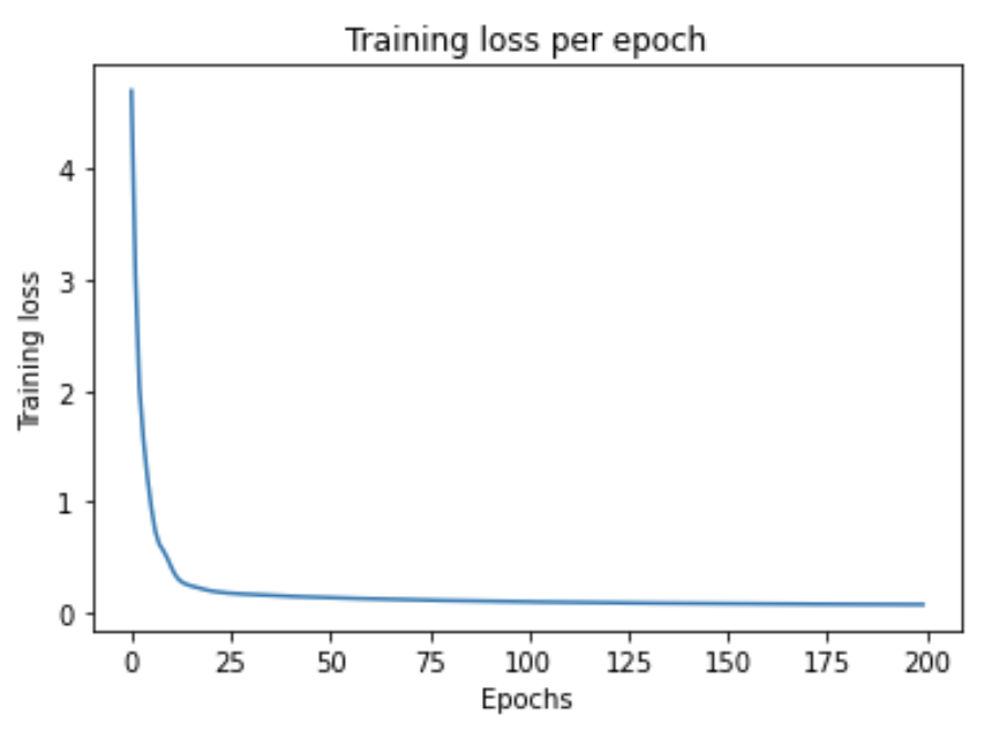
Figure4: Training loss versus epochs for BOW + voting records
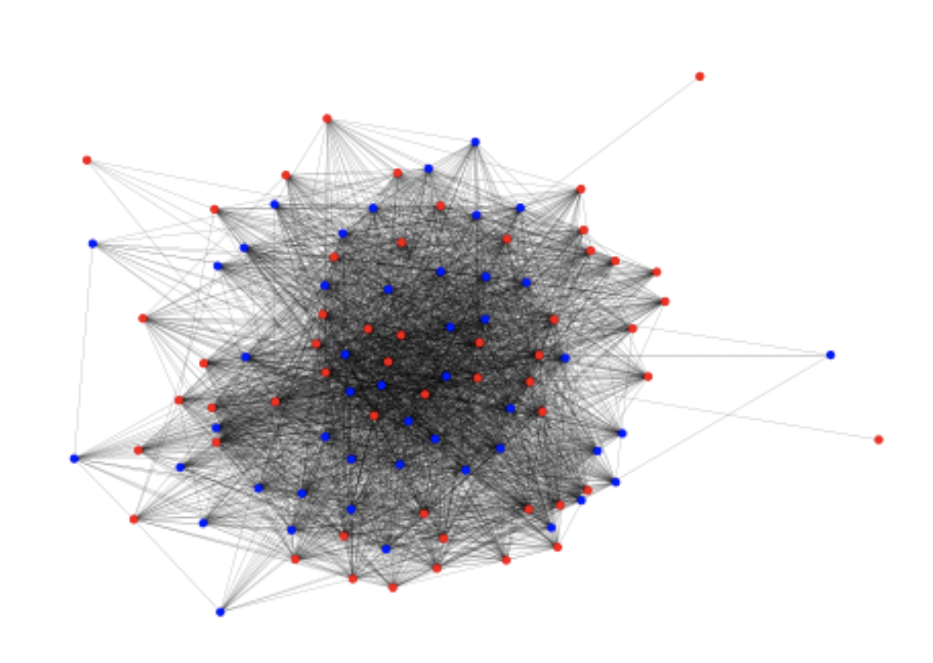
Figure5: The graph of edges after training with the GCN model. The red nodes represent republican, while the blue nodes represent democrats.
GraphSAGE

Figure6: The way to call the model and different hyperparameter for GraphSAGE model
Similar to the GCN model, A, features, labels represent the adjacency matrix, features like bag of words of Tweets and voting patterns, and political leaning of each senator respectively. And we choose to use the mean aggregator for the GraphSAGE model. Other hyper-parameters like len_walk, learning rate, num_neigh are introduced in the 4c section.
The following table shows different outcomes of the model by different features and hyper-parameters. If we use the numerical format of the text and the voting records as features, there will be 1079 features for each senator. After tuning the hyper-parameters, we finally get the accuracy of 96%, with 150 length of random walk, 8 number of neighbors, 0.3 test size, 200 training epochs and 1e-4 learning rate. And we also try to use features that only contain the voting patterns only. And we found that the result accuracy is pretty good, and can get 100% after tuning the parameter. The 100% accuracy is because we extracted how 116th senators vote for the bills. Similar logic as GCN, this is caused by the factors being too straightforward and is not that meaningful to use such factors. So we decide to use combined features as our primary sources.
| Feature | length of random walk | number of neighbors | Test size | Epochs | Learning rate | Accuracy |
|---|---|---|---|---|---|---|
| BOW + Voting records | 3 | 30 | 0.3 | 300 | 1e-3 | 90.00% |
| BOW + Voting records | 5 | 8 | 0.3 | 300 | 1e-4 | 96.67% |
| BOW + Voting records | 7 | 20 | 0.3 | 200 | 1e-4 | 93.33% |
| BOW + Voting records | 13 | 10 | 0.3 | 200 | 1e-4 | 96.67% |
| Voting records | 5 | 10 | 0.3 | 100 | 1e-3 | 96.67% |
| Voting records | 15 | 15 | 0.3 | 100 | 1e-4 | 100% |
Table2: hyper-parameters and result accuracy for GraphSAGE model on different features
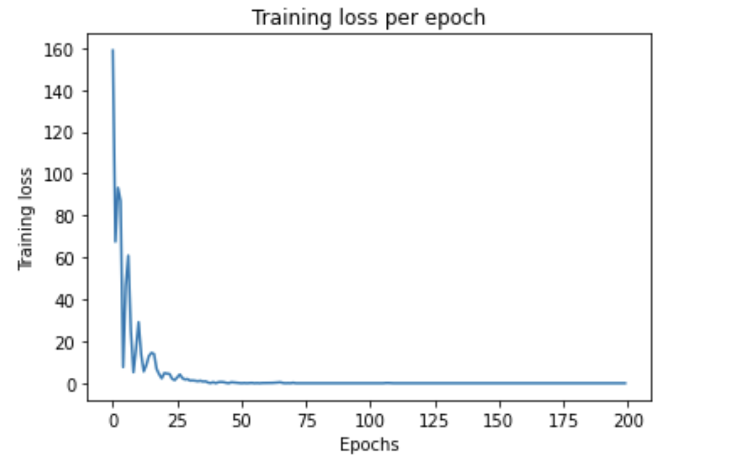
Figure7: Training loss versus epochs for BOW + voting records for GraphSage model
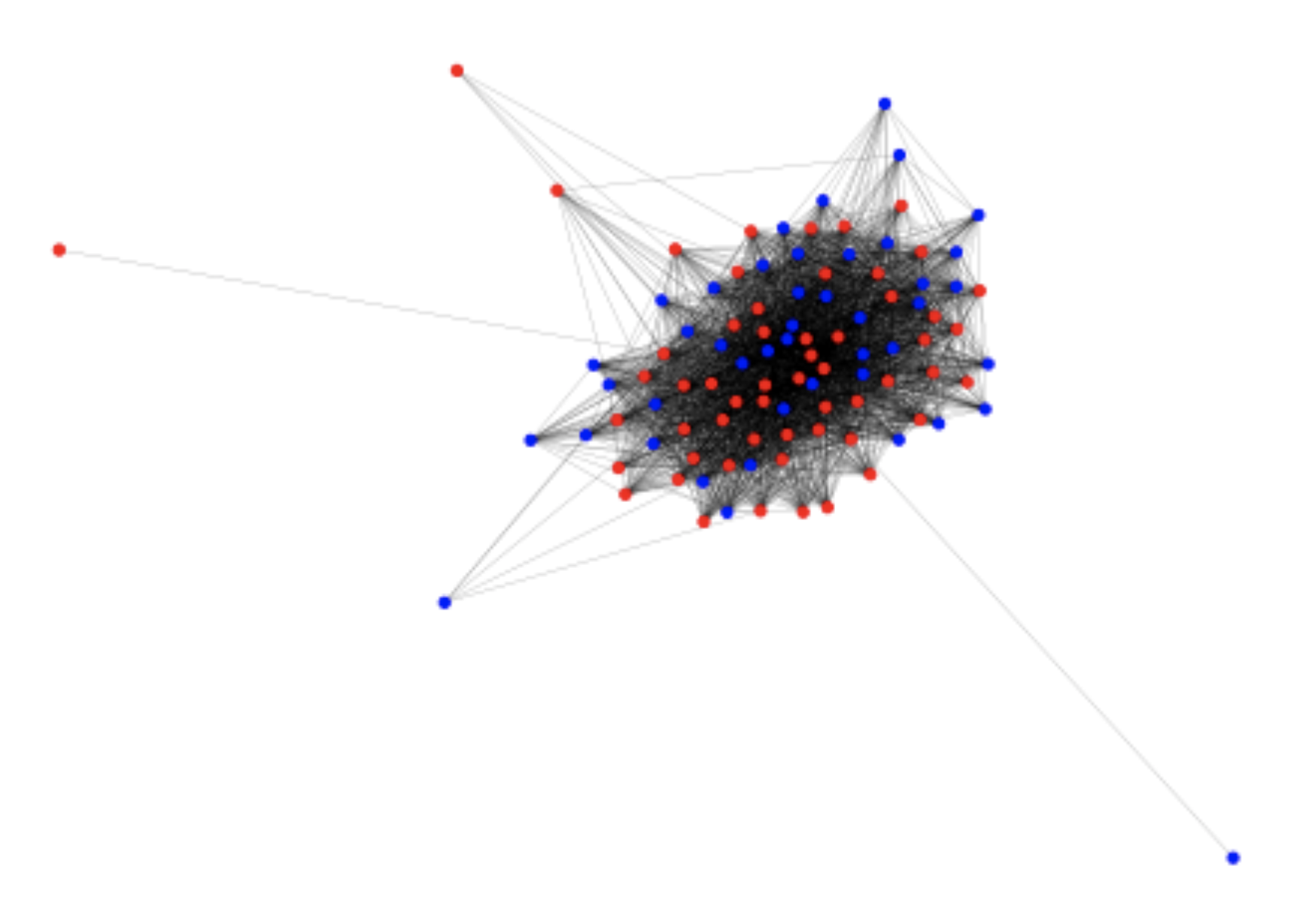
Figure 8: The graph after training with the GraphSage model. The red nodes represent republican, while the blue nodes represent democrats.
Final Result:
| GCN | GraphSAGE | |
|---|---|---|
| BOW + 116th Voting Records | 88% | 94% |
| 116th Voting Records | 100% | 98% |
Table3: Final average accuracy for GCN and GraphSAGE model on different features
Conclusion
In this paper, we predicted the senator's political party based on different features like Tweets sent by them, and voting pattern. We compared the existing graph embedding methods GCN and GraphSAGE by using similar node classification approaches. For both methods, we use different features to predict the output. The GraphSAGE model outperformed the GCN model in some runs and can provide us a relatively stable result for combined features of bag of word and voting patterns. And features using voting patterns also outperformed comparing with natural language processing on Tweets or combined features. A lot of potential improvements is possible for future work, such as extending the dataset, creating better visualization for the output, and extending the models to multimodal graphs. A further improvement could also include sentiment analysis of these tweets And one constraint we meet in this project is data extraction. If this barrier can be removed, not only the senator's political party can be predicted, we can also use the model to predict each individual's political leaning. And this will definitely be an interesting direction that can be worked with in the future improvement.